Technical Debt
Not all code is equally important. CodeScene’s strength is its ability to prioritize technical debt based on how your team interacts with the code – not just what the code looks like.
By combining Code Health metrics with development Hotspots, CodeScene pinpoints the parts of your system where poor code quality actively slows down your team, your Technical Debt Friction. These are the areas that matter most – and where refactoring delivers the biggest impact.
Prioritizes based on how you work with the code, not just the code itself. This is a crucial difference from traditional static analysis tools: some technical debt may be neither urgent nor impactful. Fixing that debt could be wasteful. Instead, CodeScene understands how your codebase evolves and prioritizes based on the organizational impact.
Limits recommendations to what’s relevant and actionable. With CodeScene, you’ll never get a list of 5.000 items to fix. Instead, you get a view of the most impactful technical debt. This allows you to balance improvements vs new features.
Automatically adapts to changing priorities and focus. Changing focus in your product development means that new hotspots emerge. CodeScene adapts automatically, updating its refactoring recommendations to what’s important for you now.
Visualize Code Health
By default, CodeScene calculates the code health of all the files in your code base.
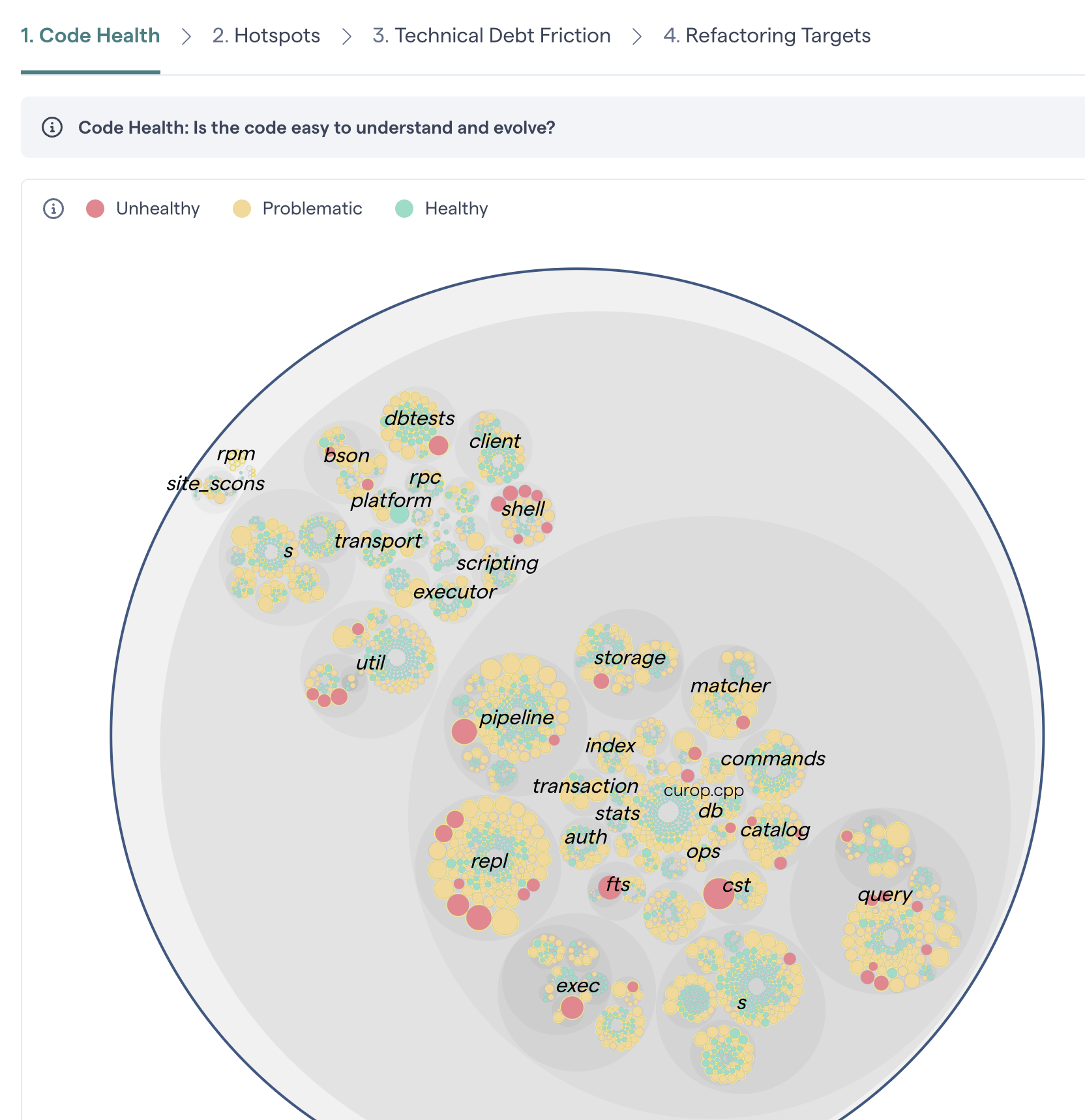
Fig. 28 View the code health of each file in your codebase.
Viewing the full code health perspective also highlights the importance of priorities. Even if a module has a lower health, that does not mean that it requires attention or immediate action. Code quality has to be put into perspective, which is something CodeScene’s other analyses do. Let’s look at some examples.
First, use CodeScene’s priorities – our machine learning algorithms will sort out the relevant code health issues from the ones with less priority.
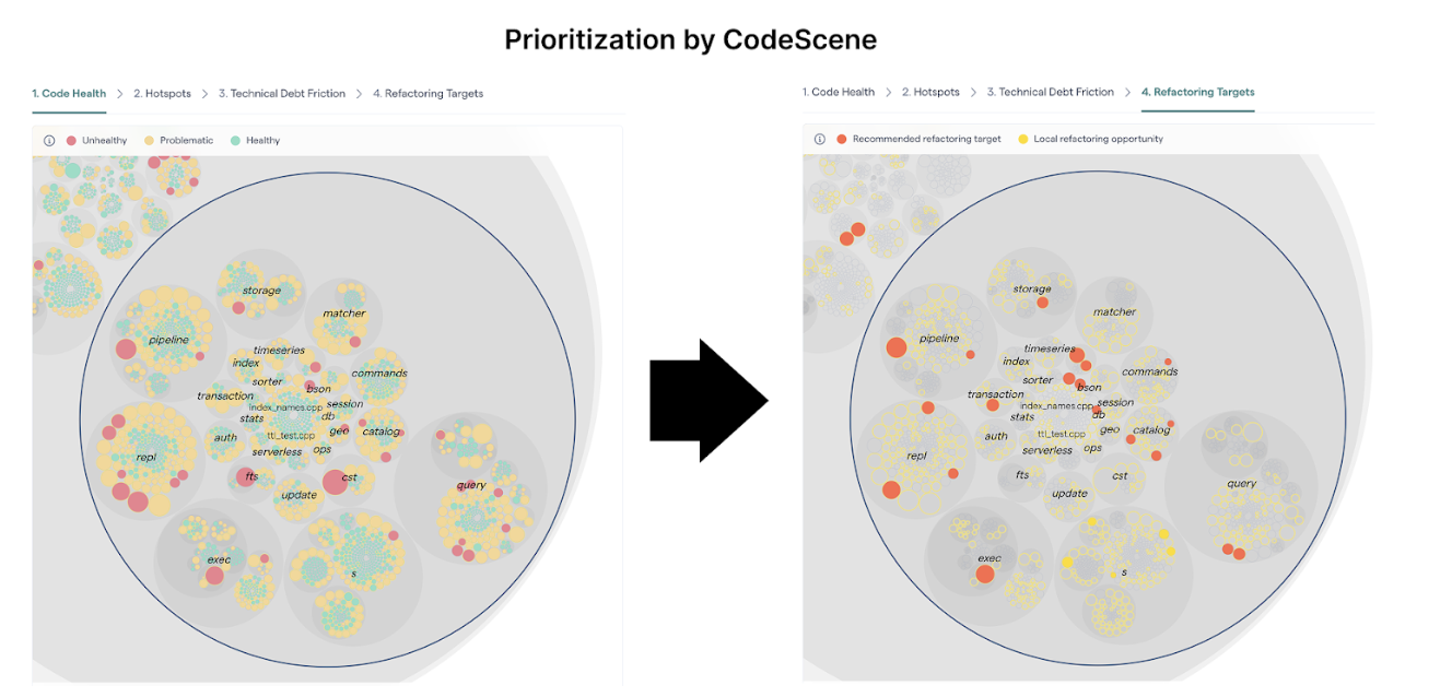
Fig. 29 CodeScene prioritizes the most relevant code health issues automatically.
Optionally, you can use the slider in the hotspot view to inspect the code health of the most active parts of the code.
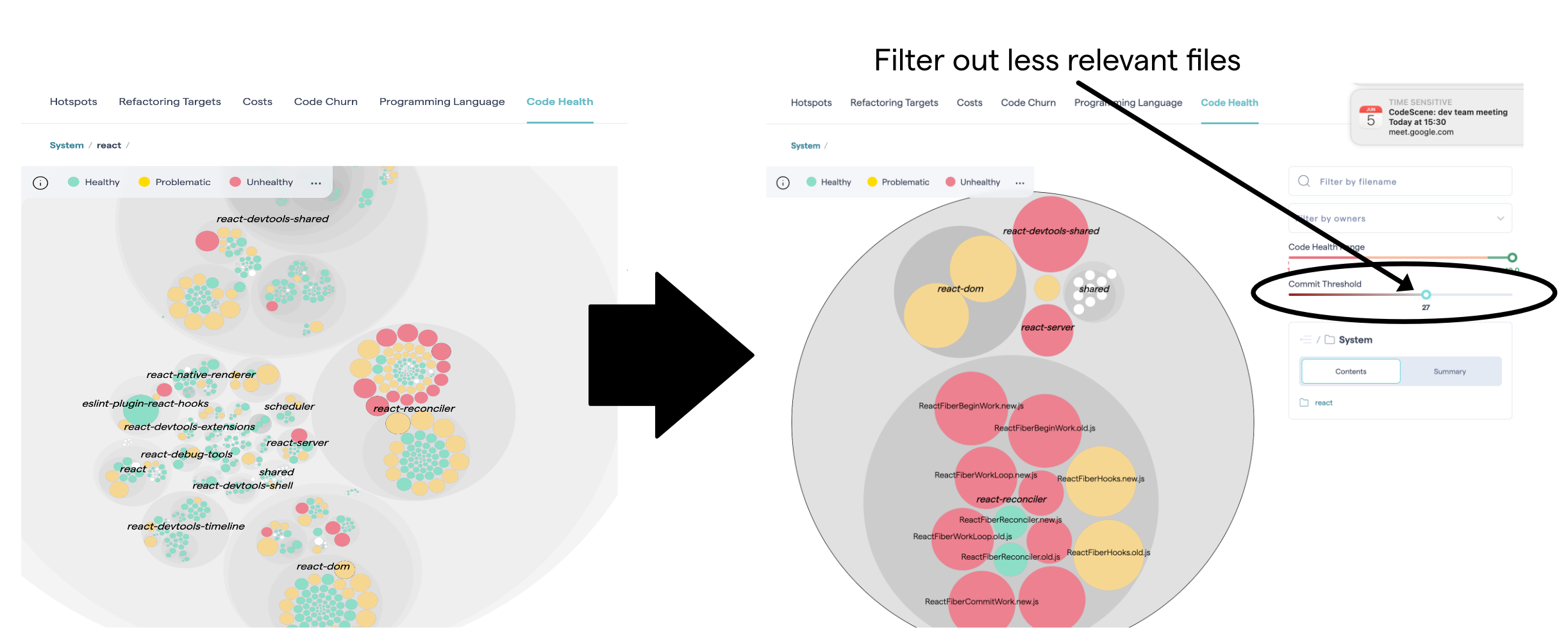
Fig. 30 Filter the code health view based on development activity.
What is a Hotspot?
Most development activity tends to be located in relatively few modules. A Hotspot analysis helps you identify those modules where you spend most of your development time.
Combined with CodeScene’s code health perspective, you can quickly prioritize technical debt or other code quality issues:
Low code health in a development hotspot is expensive. Prioritize improvements here.
Low code health in stable parts of the codebase, i.e. non-hotspots, has lower priority.
Hotspots are an excellent starting point if you want to find your productivity bottlenecks in code.
A large codebase will contain many different hotspots. Often, there will also be clusters of hotspots. Clusters may indicate that an entire component or package is undergoing heavy changes.
The visualizations on this page are available from the analysis menu at “Code > Technical Debt” or by clicking on “View Hotspots” on the “Code Health” tab of the main analysis dashboard.
Know how to use Hotspots
The Hotspots map in CodeScene is a flexible analytic tool that can be adapted to your specific needs. This kind of visualization is used in several other places inside CodeScene, so it’s worth learning how to use these maps, which we refer to sometimes as System Maps.
A Hotspot Map has several use cases and also serves multiple audiences like developers and testers:
Developers use hotspots to identify maintenance problems. Complicated code that we have to work with often is no fun. The hotspots give you information on where those parts are. Use that information to prioritize re-designs.
Hotspots point to code review candidates. At CodeScene we’re big fans of code reviews. Code reviews are also an expensive and manual process so we want to make sure it’s time well invested. In this case, use the hotspots map to identify your code review candidates.
Hotspots are input to exploratory tests. A Hotspot Map is an excellent way for a skilled tester to identify parts of the codebase that seem unstable with lots of development activity. Use that information to select your starting points and focus areas for exploratory tests.
Navigate the CodeScene Hotspot Map
The hotspots map is interactive and hierarchical. Each large blue circle represents a folder in the codebase. That means you can zoom in and out to the level of detail you’re interested in.
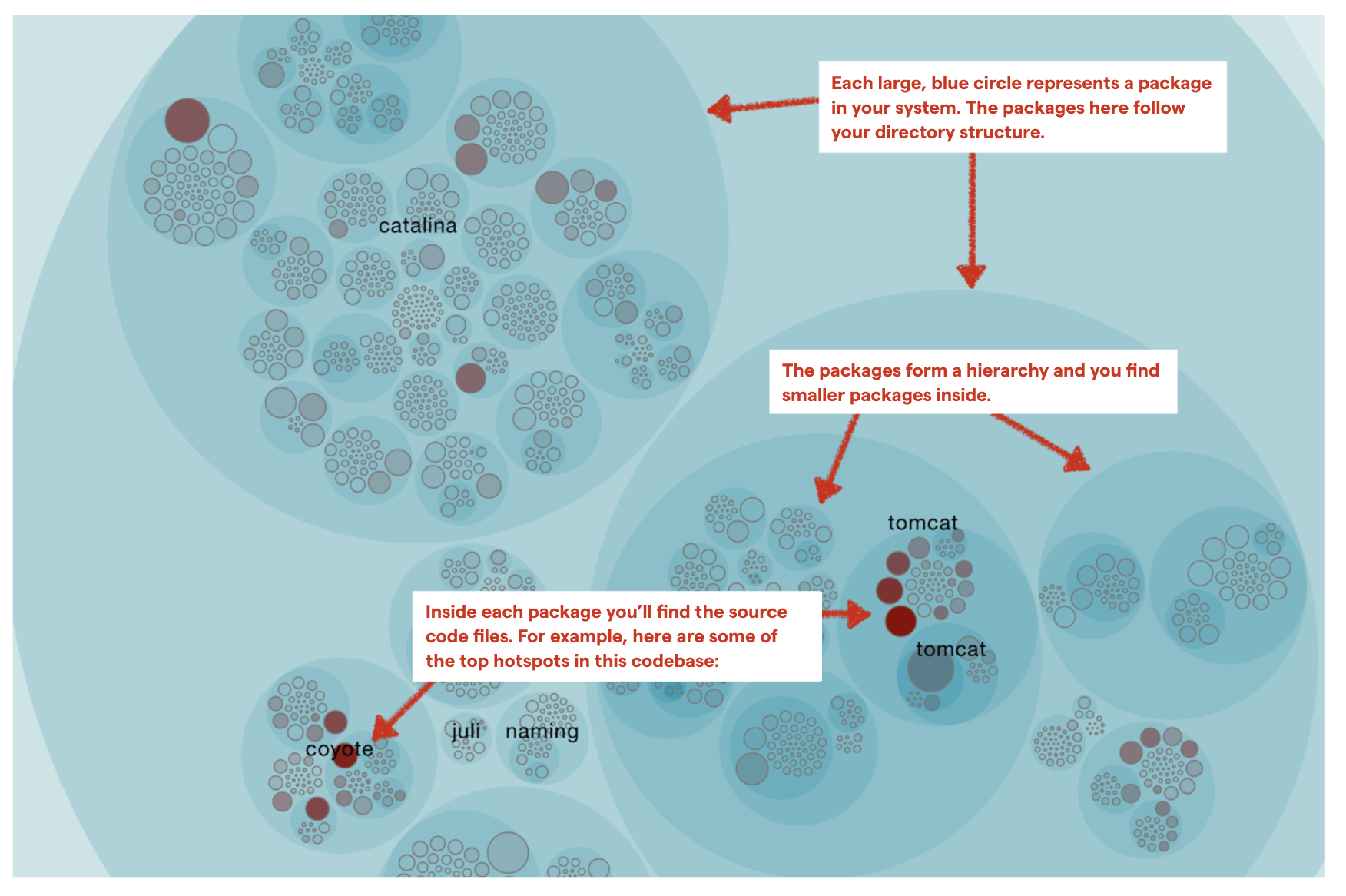
Fig. 31 Hotspots show you the activity in your codebase.
To zoom in and out, you can:
click on a directory or file circle;
scroll with your mouse wheel;
use pinch-to-zoom gestures;
click on the breadcrumbs at the top bottom of the view;
click on subfolders in the “Content” tab of the node details in the sidebar.
You can also “grab” the system map with your cursor to pan left, right, up or down.
When you click on a circle, you’ll see information about that file or directory in the sidebar, as illustrated in Fig. 32.
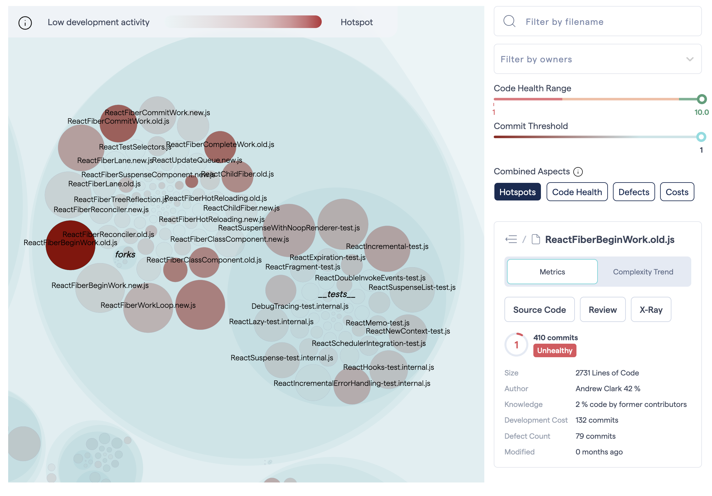
Fig. 32 Click on a Hotspot to access the context menu.
Use the context menu to access the code for inspection, run CodeScene’s X-Ray (see X-Ray), investigate trends (see Complexity Trends) and contributors (see Parallel Development and Code Fragmentation) .
CodeScene’s hotspot view also lets you view different aspects of your system, as illustrated in Fig. 33.
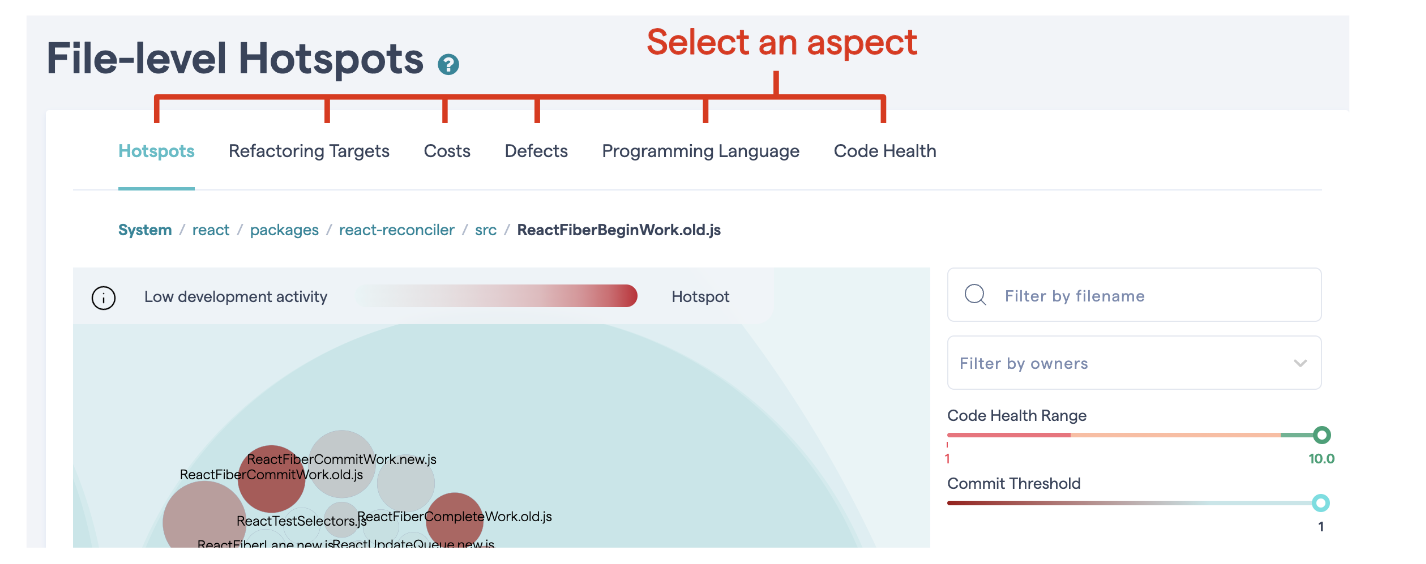
Fig. 33 Switch between different aspects in the hotspot view.
Just click on an aspect to view its data. For example, Fig. 34 shows the distribution of programming languages used in the implementation of a system.
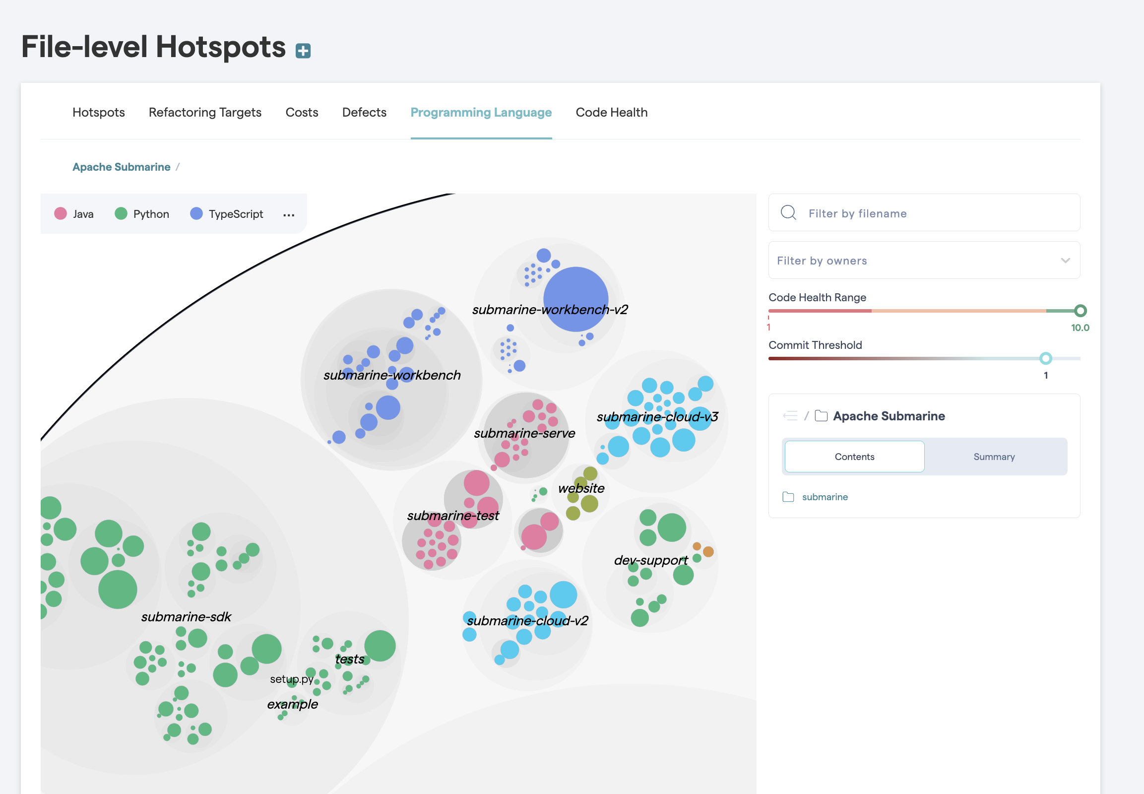
Fig. 34 The programming language aspect shows the technical sprawl in your codebase.
Deepen your analysis with combined aspects
The Hotspot tab is our recommended starting point. With the Combined Aspects feature, it helps the team building a shared mental model of what the code looks like, and where the weak and strong parts are.
The Combined Aspects are available as buttons on the default “Hotspots” tab of the Hotspots system map. When you select a button, the corresponding metric is included in calculating the color density of each file in the map.
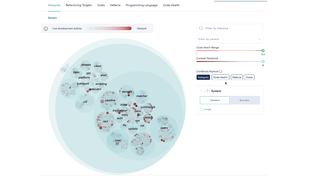
Fig. 35 Hotspots let you visualize large codebases by combining a code health perspective with temporal and organizational data.
This allows you to combine different criteria to easily identify the most interesting hotspots.
Hotspots: This is the relevance of the findings – the priority. The metric is calculated from the development activity in the code.
Low Code Health: This is the severity of any hotspot. The lower the code health, the more red the corresponding circle that represents the hotspot.
Defects: Defects are calculated from a project management tool like Jira. We explain this integration in more detail below.
Costs: Development costs are calculated from a project management tool like Jira. See X-Ray Integrate Costs and Issues into CodeScene for more details.
CodeScene caches your selected combinations in your browser, meaning you can define your own hotspot perspective based on the KPIs that are important to you.
Review your Findings: CodeScene’s Virtual Code Review
CodeScene’s virtual code review presents the code health findings, together with other module level analyses that let you investigate any hotspot.

Fig. 36 Get a holistic overview of your hotspot.
Using CodeScene’s see Code Health – How easy is your code to maintain and evolve?, you’re also able to get a quick classification on possible maintenance issues.
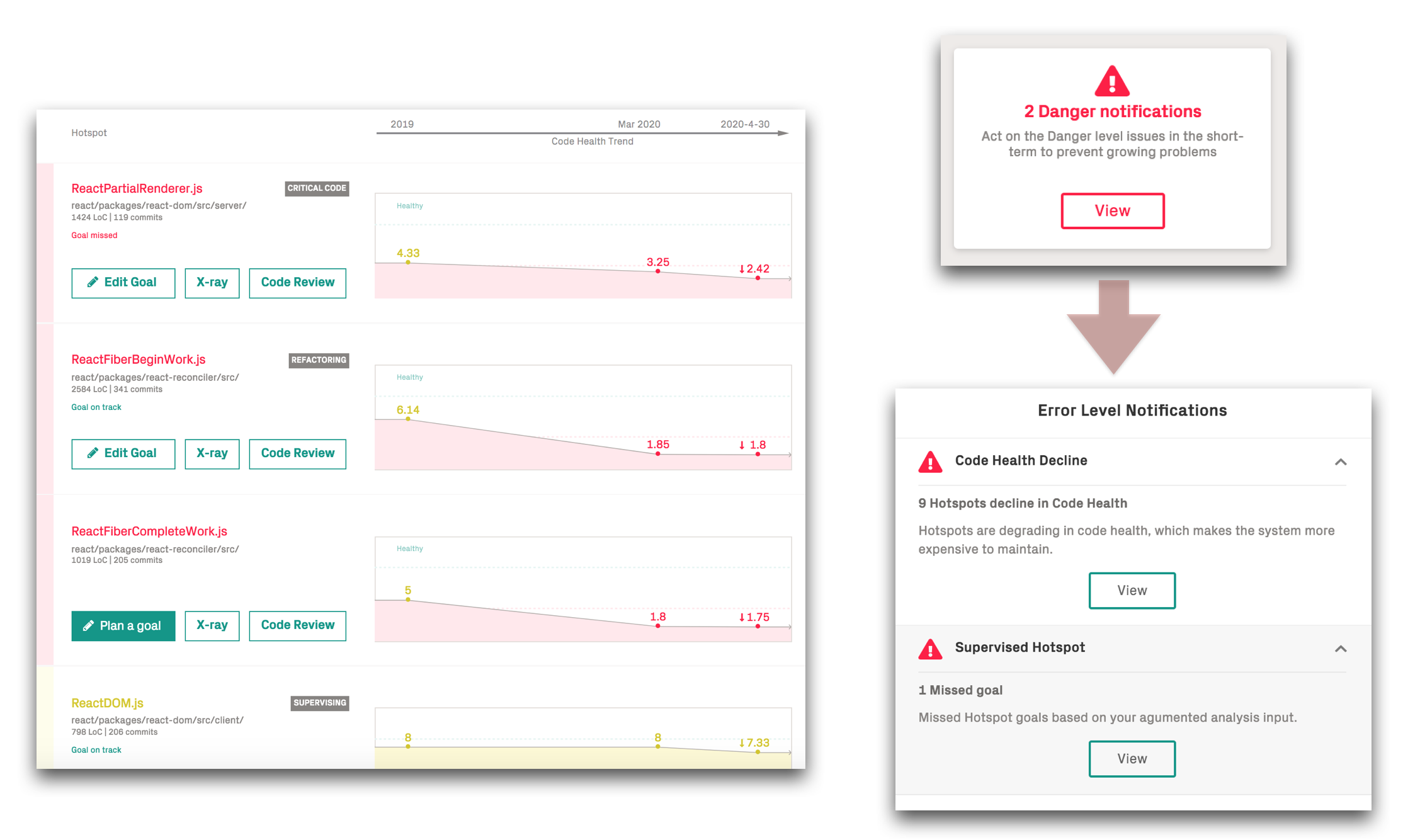
Fig. 37 View the Code Health trends for your hotspots.
The main advantage of using hotspots to guide improvements is that you’re able to narrow down refactorings to a small part of the system. That in turn will give you more time to tackle larger issues once you’ve made these initial improvements.
Technical Debt Friction
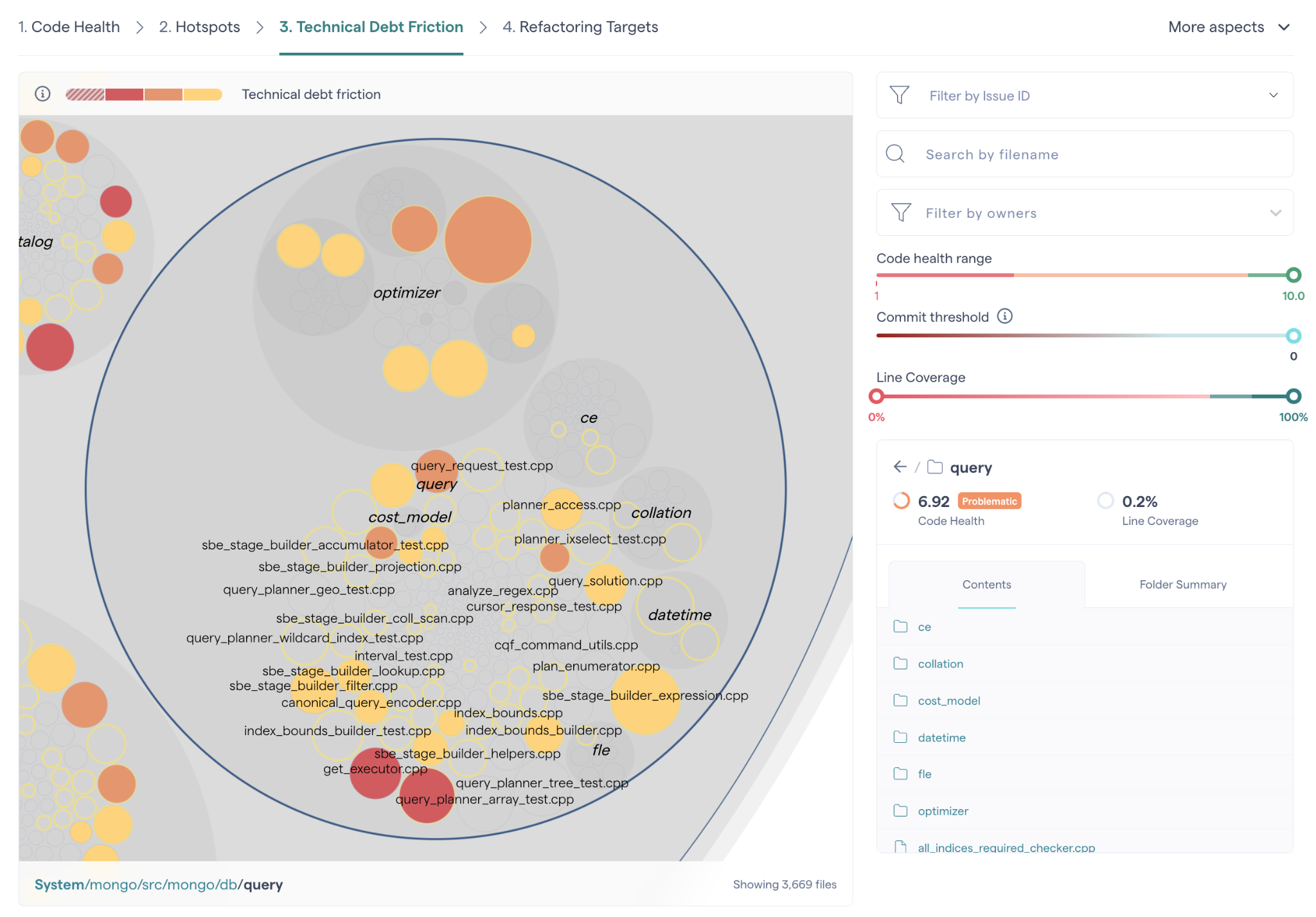
The Technical Debt Friction view helps you answer the critical question: Where is productivity hurt the most in your codebase?
This view builds on top of CodeScene’s Code Health and Hotspot analyses to identify the places where technical debt has the largest organizational impact. Unlike traditional static analysis tools that only look at the code itself, CodeScene also considers how you work with the code - how often it changes, who touches it, and how it evolves over time.
Some technical debt may exist without being urgent or impactful. Fixing that debt could be wasteful. Instead, Technical Debt Friction highlights the areas where unhealthy code intersects with high development activity, making it clear where remediation efforts deliver the biggest payoff.
Filter Hotspots interactively by Team or Developer
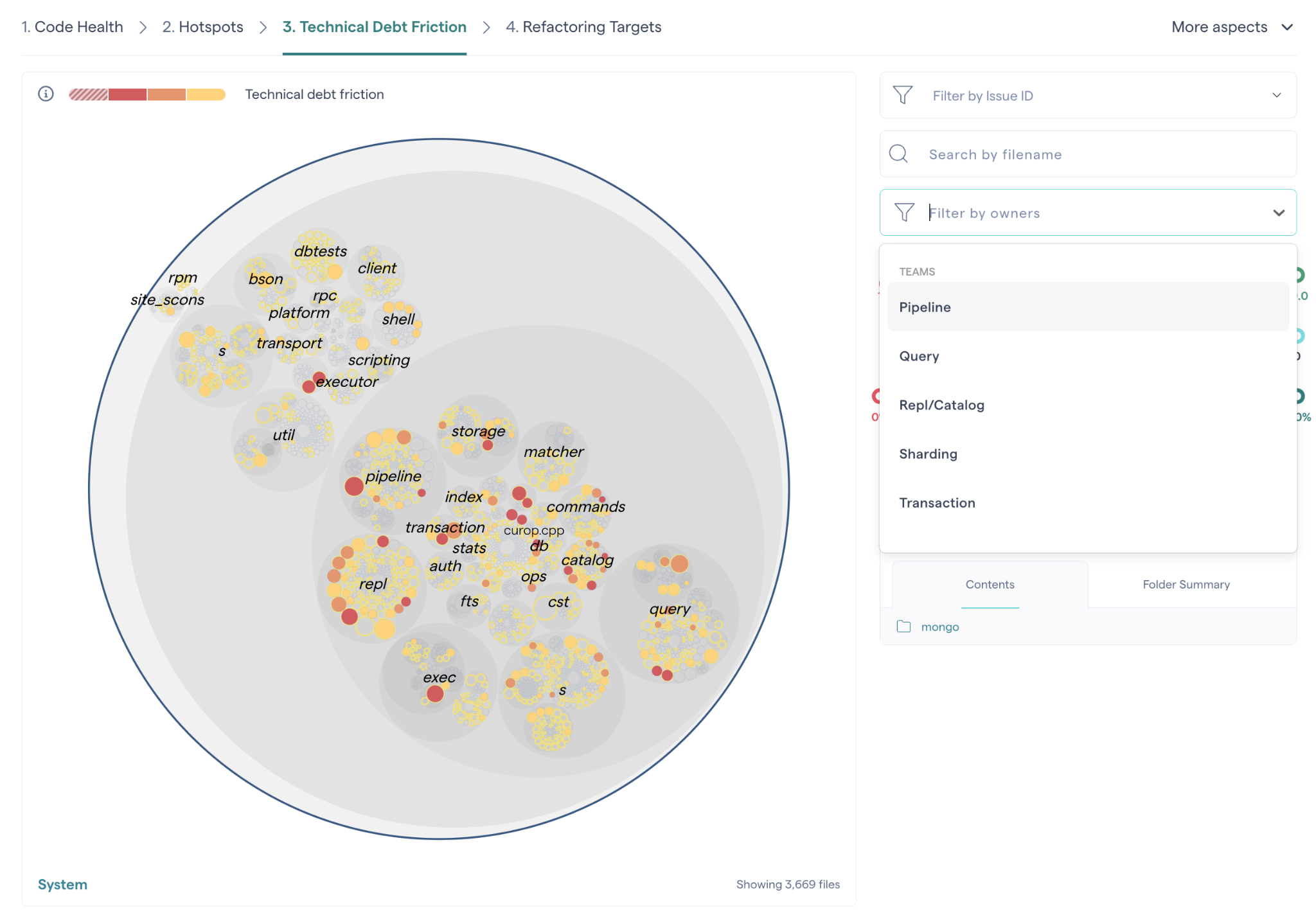
It’s common to have multiple development teams committing to the same codebase. The interactive hotspot system map lets you filter the view by team or authors. That way, you can limit the information to what’s relevant to your team.
Focus on your Refactoring Targets
To prioritize hotspots, CodeScene employs algorithms that look at deeper change patterns in the analysis data. CodeScene starts by identifying files with high change frequency and low Code Health.
Then CodeScene factors in other aspects. Complicated code that changes often is more of a problem if:
The hotspot has to be changed together with several other modules.
The hotspot affects many different developers on different teams.
The hotspot is likely to be a coordination bottleneck for multiple developers.
This algorithm allows CodeScene to rank and prioritize the hotspots in your codebase as illustrated in Fig. 38.

Fig. 38 CodeScene prioritizes the Hotspots in your code.
Red refactoring targets should be dealt with first. Remediating technical debt or code quality issues in the red refactoring targets is likely to quickly produce a real return on your refactoring investment.
Local refactoring opportunities identify technical debt remediations on an Architectural Component level which can be helpful for teams owning specific parts of a larger project.
Use the hotspot’s Code Health to get a quick assessment of potential technical debt or maintenance problems as shown in Fig. 39. We talk more about Code Health in the next section.

Fig. 39 CodeScene prioritizes the Hotspots in your code.
Once you’ve addressed those hotspots, the yellow hotspots become interesting as well. A yellow hotspot is secondary target with lower priority than the red category.
Use Defects to put Costs on Hotspots
There’s a strong correlation between Hotspots and software defects.
When you come across hotspots with severe maintenance issues, there’s always going to be a trade-off: do we pay-off the worst technical debt or should we continue to shoehorn yet another feature into the hotspot? Ideally, we would like to know for sure that if we invest, say, two weeks into refactoring the code, then that effort will pay-off immediately. At the time of writing, there’s unfortunately no way of looking into the future. What we can do instead is to look at the existing costs and consequences of not doing any preventive and pro-active code improvements.
For this purpose, CodeScene comes with a Defect Density view. Since most organizations have a known and estimated number on how much a defect costs, let’s use defects to predict the costs of any sub-optimal code we might find in our hotspots. Fig. 40 shows an example from CodeScene’s dashboard.
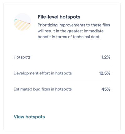
Fig. 40 CodeScene’s dashboard displays the bug density of the prioritized hotspots.
The statistics on the dashboard tells us the following things about the development costs in our codebase:
The prioritized hotspots only make up 1.2% of the total codebase, yet
we spend 12.5% of our development efforts in those hotspots, and
45% of all bugs that we detect and fix are in that small part of the code.
It can come as a surprise that almost have of all bugs, 45%, are located in 1.2% of the codebase. However, this is an extremely common situation and demonstrates the effectiveness of the hotspot as a diagnostic took. This also has direct implications on the costs of the whole system.
CodeScene’s Defect Density view shows how distributed our bug fixes are, which lets you correlate defects with hotspots as shown in Fig. 41.
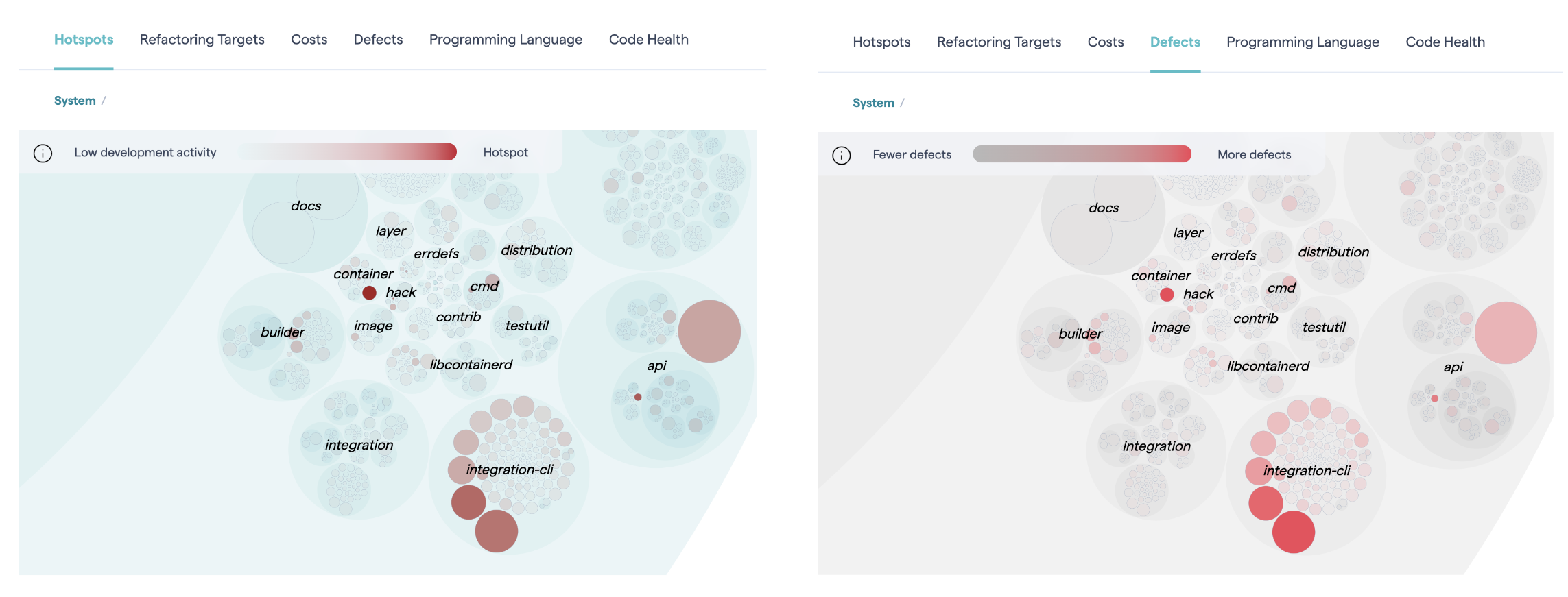
Fig. 41 Correlate prioritized hotspots with the distribution of defects in the codebase.
Specify the Data Source for Defect Statistics
CodeScene needs a data source for its defect mining, and provides two different options depending on what data you have:
Use issue types to identify defects: This requires a that you integrate a PM tool with CodeScene. CodeScene will then use all issues identified as defects for its statistics. Specify this option in CodeScene’s Project management integration as described in PM configuration.
Use commit message patterns to estimate defects: If you have specific tags in your commit messages that can be used to identify defects, then this is a good option. As a fallback, CodeScene can use a heuristic that you can override that with more specific patterns for higher precision, as shown in Fig. 42.
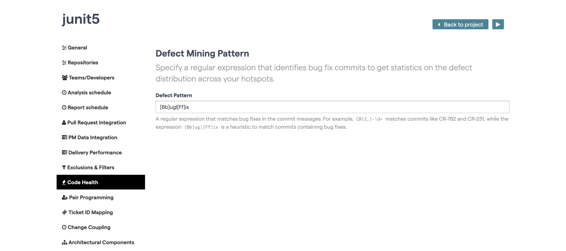
Fig. 42 Configure a pattern to match defect information in your commit messages.
This configuration item can be found in the “Code Health” tab of the project configuration.
Visualize relationships between files with change coupling
CodeScene identifies files that tend to change together. Change coupling indicates a relationship of some kind between files. These relationships are visible in the hotspot map when you hover your cursor over a file with coupling.
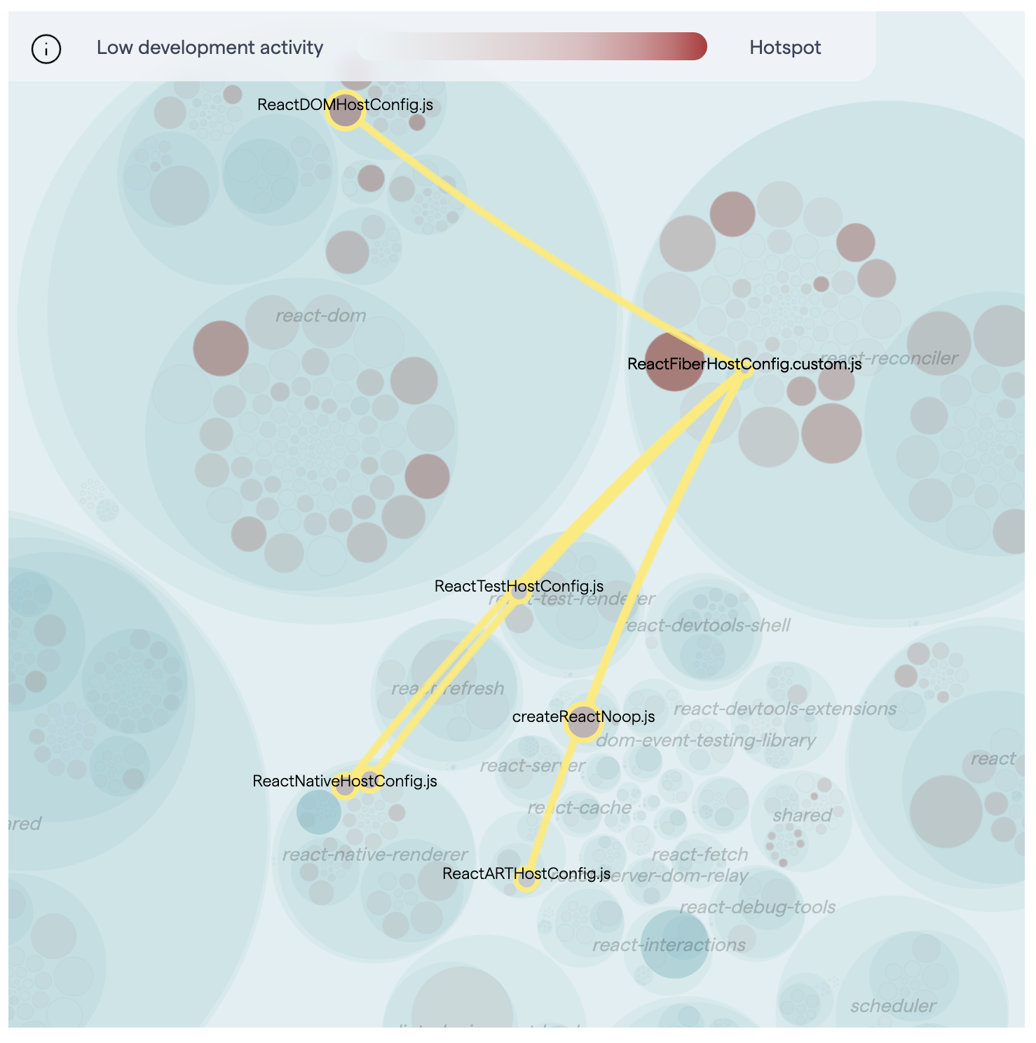
Fig. 43 Hover over a file to see its connections to other files.
Interpreting change coupling depends on the context. Widespread change coupling in a codebase can indicate tightly coupled logic and possible architectural issues, like in this example.
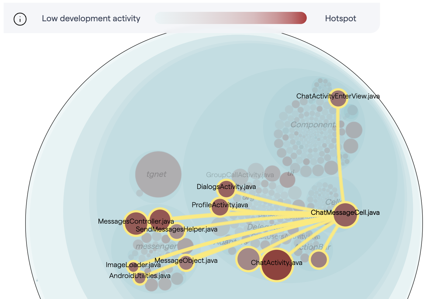
Fig. 44 A tightly coupled codebase.
Making a change in one of these files often means making changes to the others as well. It’s easy to imagine how these interdependencies complicate things for developers who need to fix bugs or add features in any of those files. In this case, change coupling is problematic.
Change coupling can also be positive, when it occurs between files that have a good reason for changing together. This is the case with test code, like in this example.
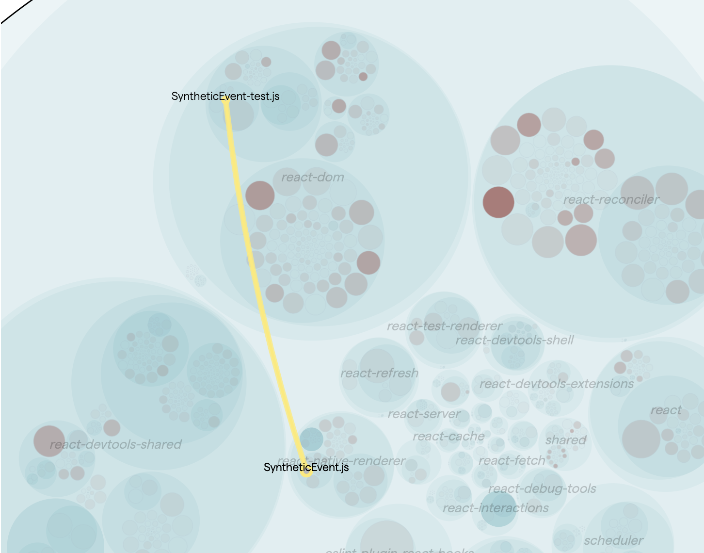
Fig. 45 Change coupling between a file and its tests.
There is coupling between SyntheticEvent.js and its test file: SyntheticEvent-test.js. This is a positive sign that suggests that the tests are being updated as the file evolves.
Hovering over files with change coupling causes the coupling lines to appear for as long as you hover. This can be inconvenient if you want to zoom out or shift the viewport to see the rest of the map. In that case, clicking will “lock” the change coupling visualization, leaving you free to continue to interact with the system map.
There are two other consequences when this happens:
When one file is “locked”, hovering over other files still works. In this case, the coupling lines are white, in order to differentiate them from the first set of couplings.
When a file with change coupling is selected, a third tab will appear in the sidebar, providing detailed information about the different change couplings.
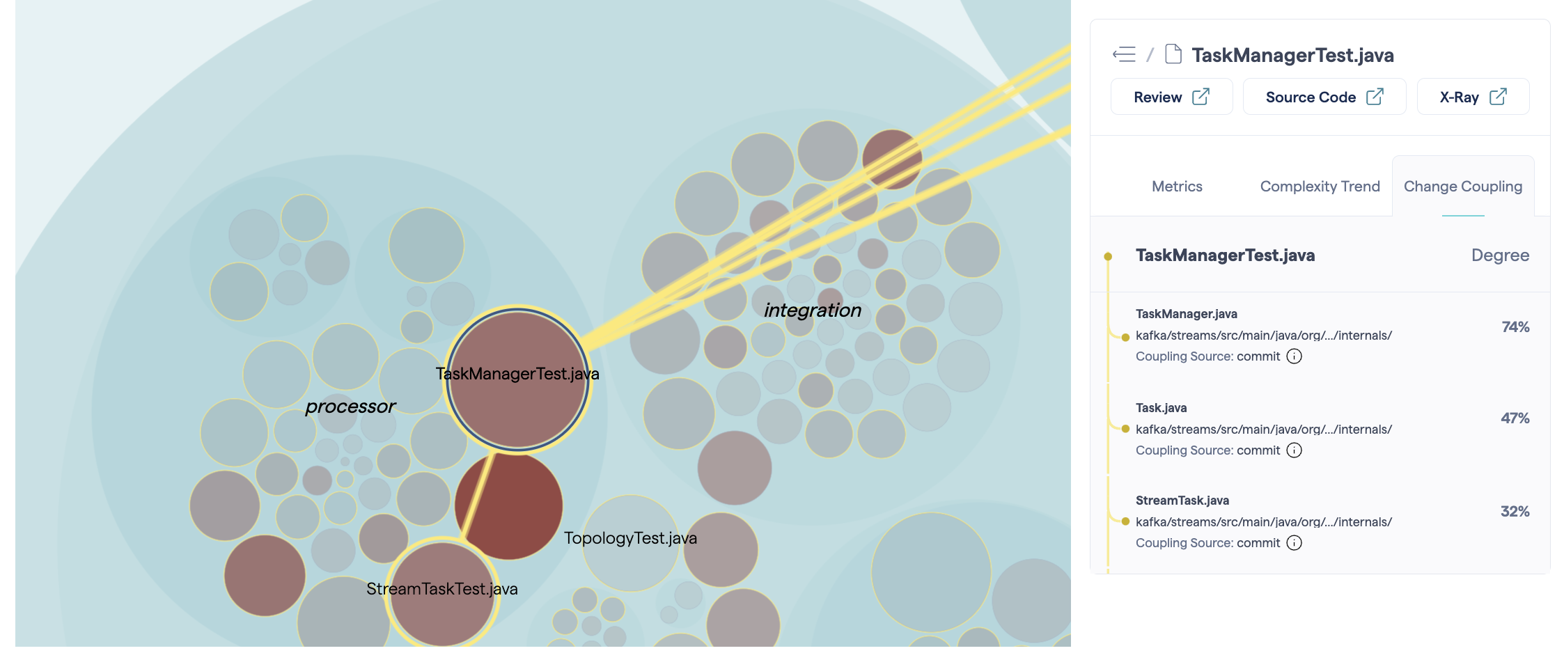
Fig. 46 With a file locked, the change coupling sidebar appears.
The “Degree” indicates the strength of the coupling. (For more information about how the couplings are calculated, see Change Coupling: Visualize Logical Dependencies.) The “Coupling Source” identifies how CodeScene identified the change coupling. The system maps use two possible sources:
Commits: files are modified as part of the same commit;
Project management tool tickets: files are modified as part of the same ticket.
In general, commit-level change coupling indicates a stronger level of coupling. However, changes made in separate repositories cannot be part of the same commit, so we then turn to ticket-level change coupling, which is not perhaps as “strong” but has the advantage of seeing couplings that would otherwise remain invisible.
For more information, see Change Coupling: Visualize Logical Dependencies. The change coupling data used in the hotspot map is calculated the same way as for the other change coupling graphs, with two exceptions:
Filters are not applied. This allows “positive” coupling, like for tests, to be visible.
The coupling threshold is fixed at 20% which will generally be lower than the automatic default in the change coupling graph.