Using Code Coverage
Code coverage is a set of metrics that shows how much of your source code is executed when your automated tests are run. CodeScene allows you to visualize code coverage in your project and to track the evolution of your coverage statistics over time.
The code coverage integration becomes exceptionally powerful when combined with CodeScene’s other analyses, such as hotspots and refactoring targets, or view per team or per architectural component.
There is no such thing as a “good” coverage score – it all depends on context. For example, in a critical hotspot, you need a higher degree of coverage to refactor safely, whereas you can get away with lower coverage in stable and well-understood parts of the codebase. CodeScene provides those priorities to put coverage metrics into context.
When code coverage is enabled, the data appears in three separate views:
All of these are documented below. First, however, let’s take a quick look at some general aspects of code coverage in CodeScene.
Code Coverage Metrics
There are multiple code coverage metrics, and the most popular are:
Line coverage: which lines of code have been covered by automated tests?
Branch coverage: which execution paths have been covered by automated tests? For example, a line of code like
if a && bcan have full line coverage, but only partial branch coverage.
See here for a complete list of the coverage metrics and formats that CodeScene supports.
The code coverage dashboard
The code coverage dashboard is the primary source of information about code coverage in your project.
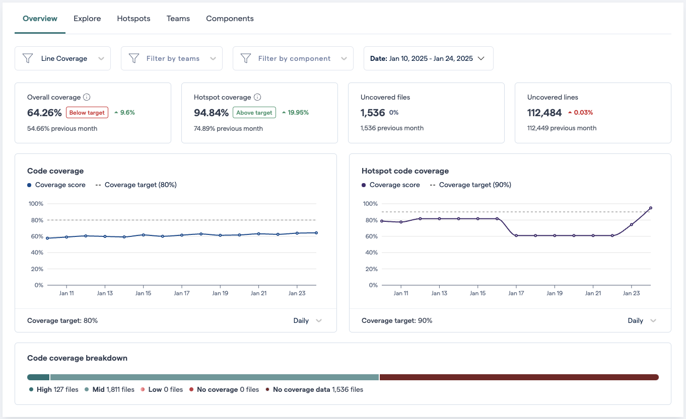
Fig. 166 The Overview tab of the code coverage dashboard
The “Overview” tab allows you to track high-level trends, while the system map in the Explore tab provides an interactive way to drill down to the file level, and to use CodeScene’s hotspot and code health metrics in conjunction with code coverage.
Overview
The Overview tab displays three different kinds of information:
High-level code coverage KPIs
Historical code coverage trends
Information about the limits of the available code coverage data.
With this view, you can get a quick idea of the current state of code coverage in the project, or use the filters to drill down into much more specific aspects.
Filters

Fig. 167 There are several useful filters.
The overview provides multiple interactive filters. These filters are applied to all of the charts and KPIs presented in the “Overview” tab, and, when appropriate, filter choices are carried over to the other tabs.
Coverage type
This dropdown menu contains the code coverage types available for the current project. Line coverage is present in all cases. The availability of the other types depends on what data has been uploaded. After you upload a new coverage type, you’ll need to run a new analysis before it appears here.
Teams and Architectural components
When the team filter or the architectural component filter is activated, you’ll see metrics derived from the matching files. For teams, this means the files “owned” by members of the team.
Note that the Teams and Architectural components filters cannot be active at the same time.
Date range
The date filter allows you to zoom in and out over different time scales. Note that this does not affect the “Explore” tab.
KPIs
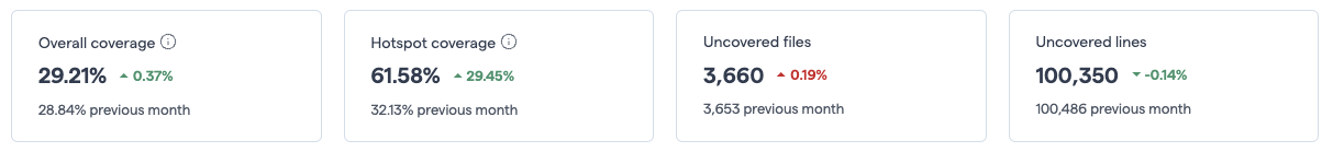
Fig. 168 The top-level code coverage KPIs
The most important KPIs can be found at the top of the page allowing for a quick view of the latest coverage status. The values shown reflect the state of the project at the end of the currently selected date range, taking into account any filters that are applied.
Overall coverage
Code coverage for the entire project. This average is calculated by taking the total number of items the metric is based on (lines, branches, statements, conditions, etc.) and comparing to the number of items that are called during tests.
Hotspot coverage
Code coverage for the files that are most actively worked on.
Uncovered files
The number of files with no coverage. For Line coverage, this total potentially includes all non-excluded files.
Uncovered lines, branches, etc.
Depending on what type of coverage is currently selected, this KPI shows how many lines, branches, conditions, etc. do not have coverage. For Line coverage, this includes lines from all non-excluded files in the project. For the other coverage types, this will only include branches, statements etc. from the files for which the coverage tool supplied data.
Charts
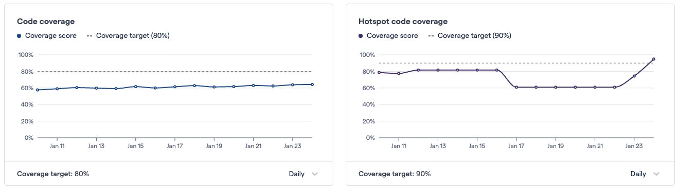
Fig. 169 The overall coverage and the hotspot coverage charts allow you to track progress over time
These charts are showing code coverage over time, for the entire project, on the left, and for hotspots, on the right.
The level of detail depends on the active date range selection. It can also be adjusted by selecting a date scale in the dropdown below teach chart. If “Daily” is selected, then the “Dec 19” value will correspond to the latest analysis run on that day; if “Monthly” is selected, then the values will be the last value for each month. As with the KPIs, the values shown are the last values for a particular time slice.
Code coverage chart
The code coverage chart tracks the average code health over time, and considers all matching files (the entire project, or the files matching the selected team or component).
For each point on the chart, you can hover to see the score at that time, along with the percentage change relative to the previous point. Clicking will reveal more possibilities for clicking through to more detailed information per-team or per-component changes. For even more detail, you can click through to the “Teams” or “Component” tabs.
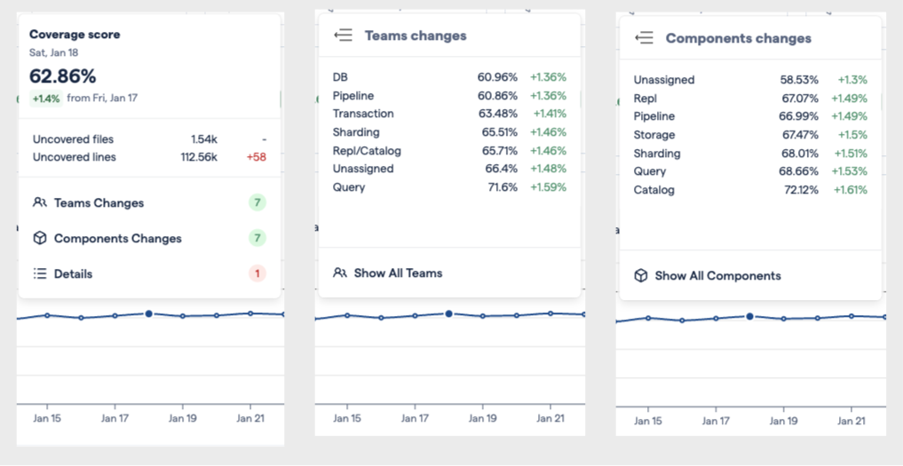
Fig. 170 These tooltips can help understand the movements in the displayed values.
The “Details” option shows more information about the state of the code coverage data.
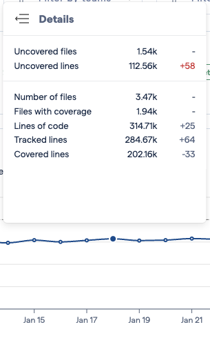
Fig. 171 The details reflect the state of your code coverage data.
Hotspot code coverage chart
The Hotspot code coverage chart shows the evolution of the code coverage scores of the most active files in the project. Since tests are a way to manage the risk associated with change, it is important to ensure that the files changing the most often have a high level of code coverage.
Because the hotspots are a very small subset of the files in a project, it is to be expected that this graph will be much more volatile than the Code coverage graph on the left. Changes, in the same direction, in the coverage score of two or three files will often be enough to cause a visible shift.
Hotspots are a moving target. As developers work in different parts of the codebase, the list of the most active files will evolve over time. Files that become more active will push the less active files out of the list. The hotspots code coverage curve reacts to these changes. At each point in time, it reflects the code coverage level of your priority files.
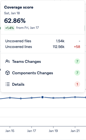
Fig. 172 How do we explain this drop in the hotspot coverage score?
The popups on the Hotspots code coverage chart can help understand why a change in the score may have occured. In the example shown here, the drop on January 17th was probably caused because of increased development activity on two new files, presumably with lower code coverage scores than the previous average. At this point, we don’t know if this is the only reason for the change, or if the coverage of other files also decreased. To get an even clearer picture, we can go to the Hotspots tab.
Information about the status of the code coverage data
Aggregating accurate code coverage data, especially for large complex projects, is not always easy. Code coverage uploads can be out of date; parts of a project may not have code coverage data at all yet. Factors like these can influence the results that are displayed.
To provide transparency into your coverage data, CodeScene warns about file mismatches and provides the Code coverage breakdown, which are described below.
File mismatches: On all the charts, in some circumstances small warning triangles will appear for one or more points in time. These indicate that when the last analysis was run, files had changed after the latest code coverage data was uploaded. This usually means that the most recent coverage data is not available, either because of upload failures or because coverage uploading is not part of your CI/CD pipeline yet.
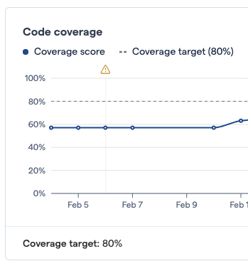
Fig. 173 On February 6th, changes were made after the code coverage data was uploaded.
If the warning occurs for the latest analysis period, it could mean that there could be a problem that should be investigated. Warnings for earlier time periods are included because the file mismatches could mean that the results are not entirely correct for the affected period.
Code coverage breakdown: The Code coverage breakdown shows the distribution of a project’s files in different code coverage categories. The different areas of the chart are weighted by file size. The values shown reflect the end of the currently selected date range.
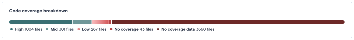
To get a better understanding on the files included in the code coverage analysis, the Code coverage breakdown will show the current state for different files.
High |
> 80% |
Mid |
40-80% |
Low |
< 40% |
No coverage |
0% |
No coverage data |
No data for these files was provided. |
The last two categories deserve some extra explanation. Depending on which code coverage tool or tools you use, it is not always possible to determine if a file has 0% coverage because it truly was never called during the instrumented tests, or if it is because no code coverage was run on that part of the codebase or on files of that language. CodeScene attempts to show this distinction when possible but it is always good to make sure that code coverage data is being generated and uploaded for as much of the codebase as possible. If there are files that, for whatever reason, cannot be analyzed by a code coverage tool, it can be helpful to use the code coverage exclusions so that those files without data do not affect your code coverage.
Explore: Visualizing code coverage in CodeScene
The Explore tab presents a system map for visualizing code coverage. The visualization will be familiar to you since it is used in many places in CodeScene, such as the Technical Debt map.
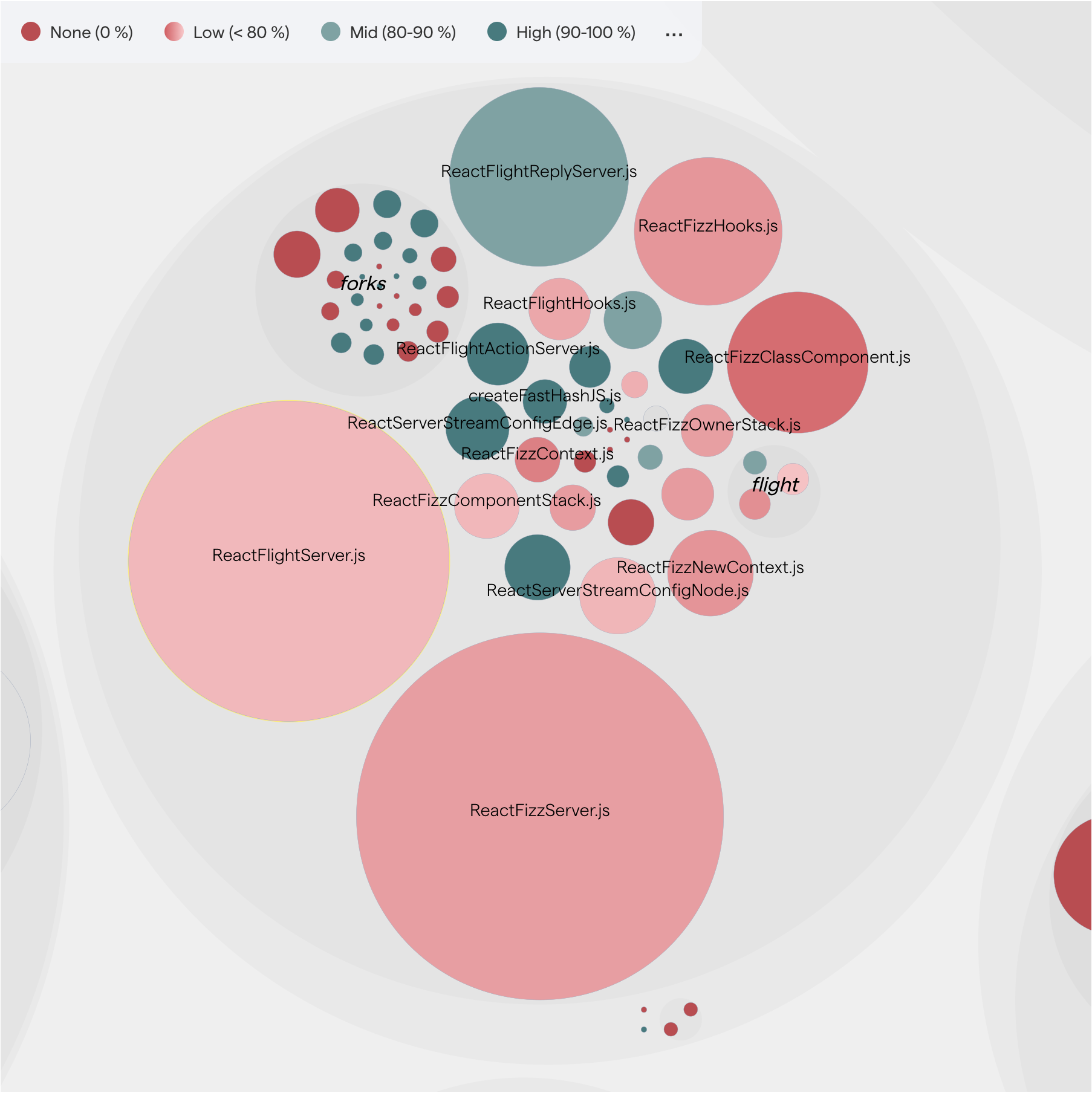
Fig. 174 CodeScene visualizes code coverage in its interactive views. The green nodes signify high code coverage, while red nodes represent low code coverage.
Note that when code coverage is enabled in CodeScene, an additional tab is also added to the main Technical Debt map. (See below for details.) Much of what is described here also applies to the Code coverage tab of the Technical Debt system map.
To view a project’s total average code coverage, click the top-level circle in the interactive Technical Debt map. The value will appear in the sidebar.
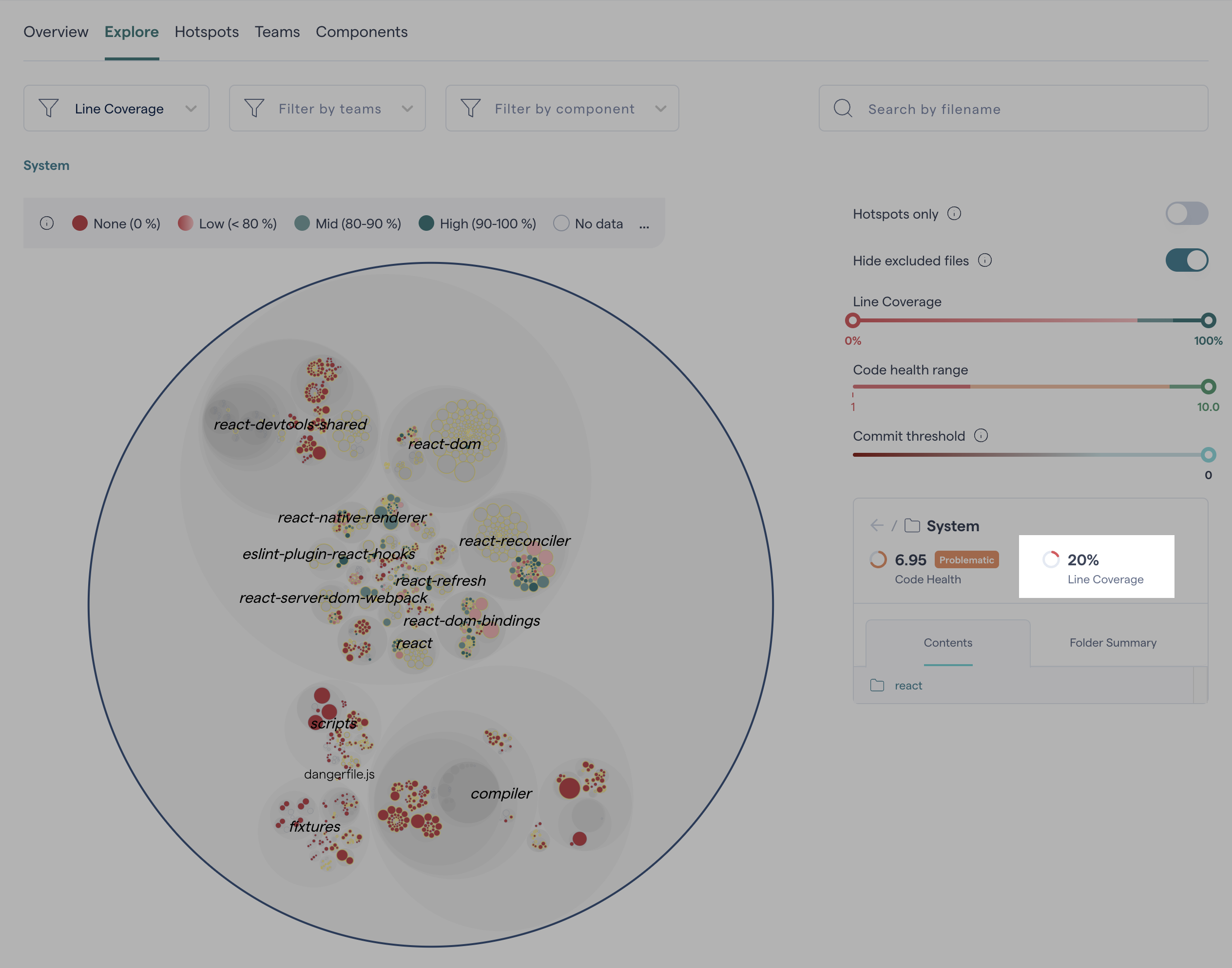
Fig. 175 The code coverage score for the selected node is displayed in the sidebar.
Quickly view the code coverage score for the most critical parts of your project, by using the Hotspots only toggle. To explore the project’s code coverage in more detail and identify areas with lower scores, adjust the Coverage Slider to filter the map and focus on areas that need improvement.
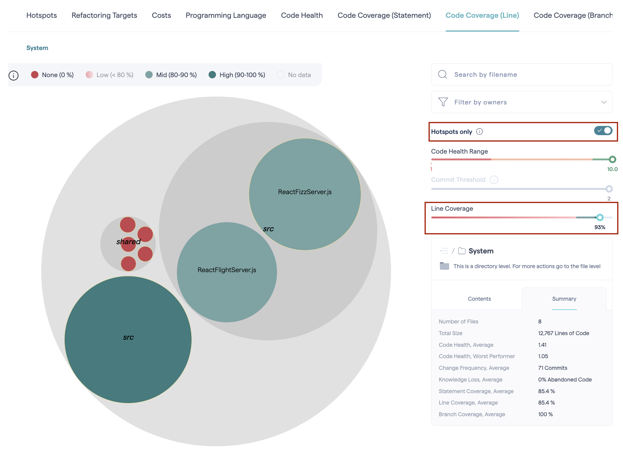
Fig. 176 Using code coverage filters.
When you click a on file, its code coverage score is shown; clicking on a folder shows the average score of all its files.
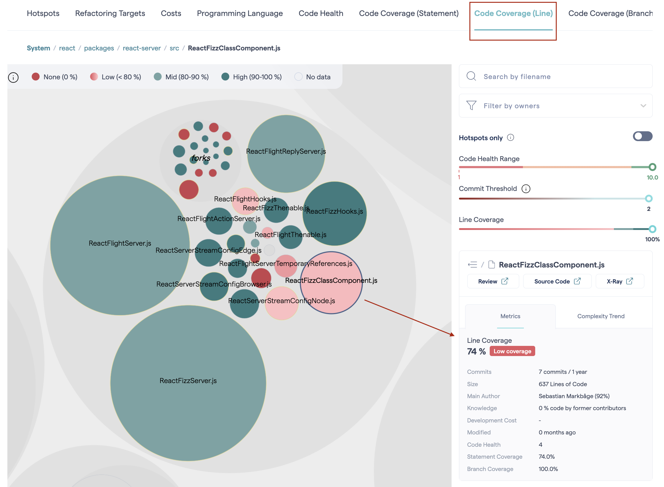
Fig. 177 A file’s code coverage score.
Together, the Coverage Slider with the Code Health and Commit threshold sliders for a powerful analytical tool.
The typical use cases are:
Prepare for refactoring: identify feature areas with low coverage before planning refactoring tasks. For example, refactoring a complex hotspot that doesn’t have adequate code coverage would be high risk.
Mitigate risk: identify complex hotspots that don’t have sufficient code coverage and plan to improve.
Hotspots tab
The Hotspots tab provides the information necessary for a detailed analysis of the code coverage status of the most active files in a project.
The data shown for each file corresponds to the point in time selected on the chart. When the tab is first opened, by default this will be the latest point. By clicking on other points, you can see the matching scores and lists of files.
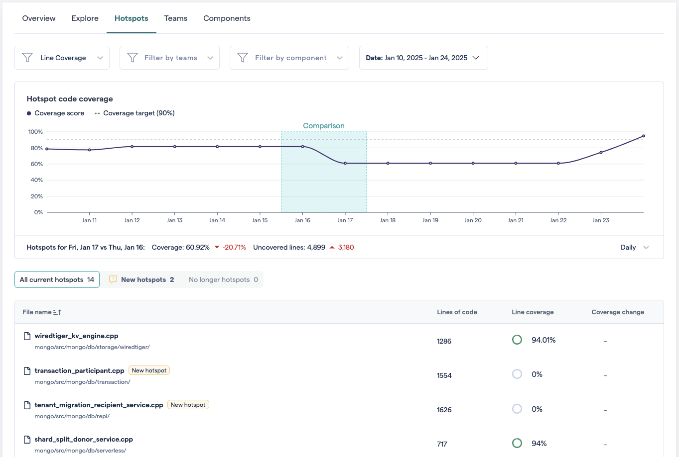
Fig. 178 The hotspots tab provides many details about what’s happening to the code coverage of your hotspots
Code coverage changes, like -20.71% in the graph below, are calculated relative the previous point in time. The “Comparison” zone helps show which points are being compared.
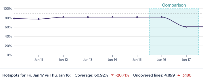
Fig. 179 Comparisons are between one point and time and the previous point.
The “New hotspots” and “No longer hotspots” filters can help understand which changes to the list of hotspots are responsible for differences in the hotspot average.
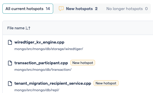
Fig. 180 Knowing which files are new hotspots can help explain changes to the average.
Teams and Architectural components tabs
The Teams and Architectural components tabs work in much the same way as the Hotspots tab, with a few small differences.
The most important difference is the possibility of displaying trends simultaneously for up to 10 teams or components. The individual teams and components can be toggled on or off in the list or by clicking on the charts legend items.
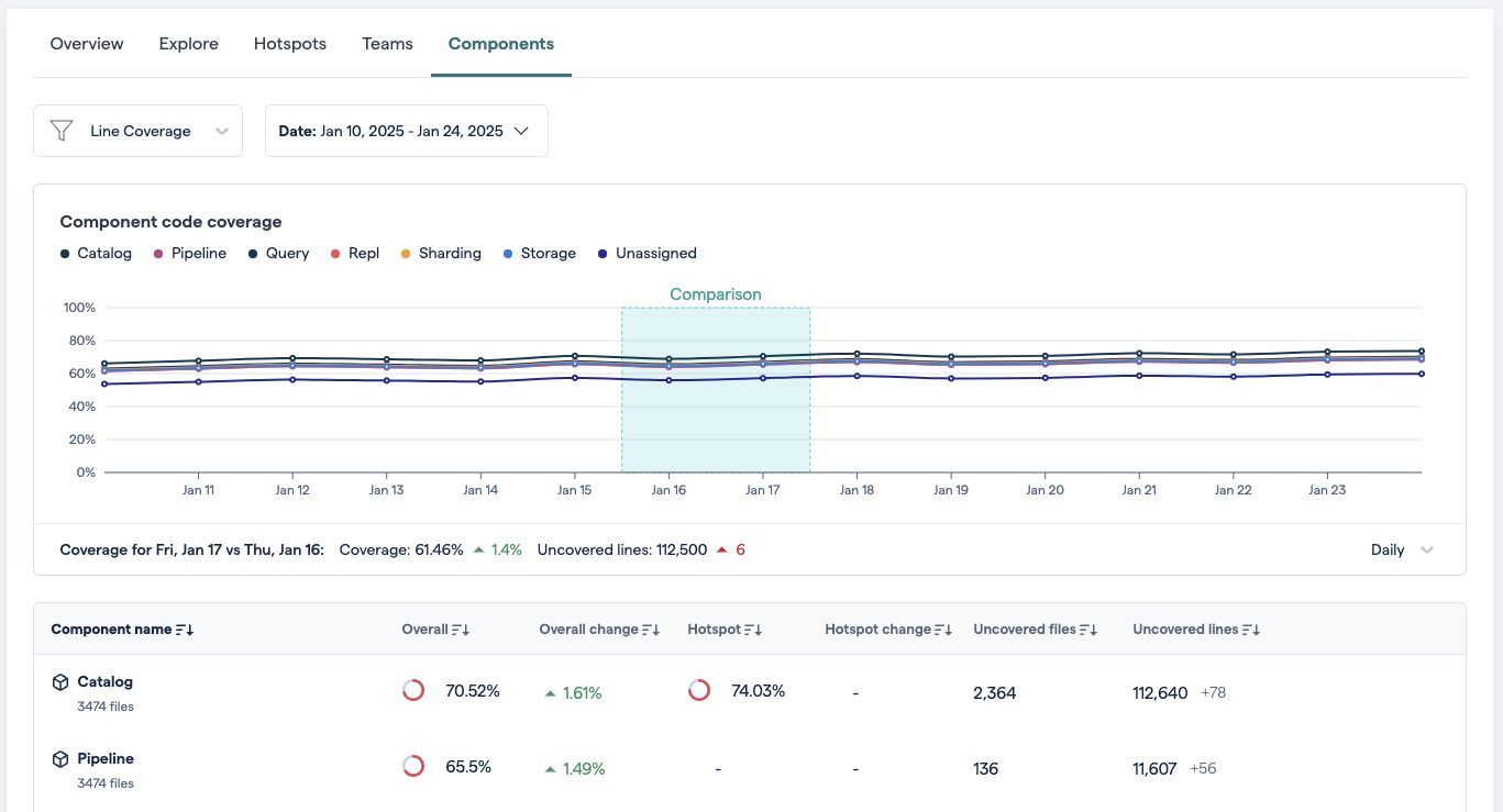
Fig. 181 Architectural components tab
Line coverage and the others
CodeScene handles Line coverage differently from the other coverage types. This is because CodeScene can estimate the total number of what most code coverage tools consider to be active lines across the entire project. CodeScene is therefore able to compare the number of covered lines, provided by the code coverage tools, to an estimation of the entire project. You can find more information about how the calculation is performed here.
For the other types of coverage, CodeScene cannot estimate the number of branches, statements, decision points etc. that the project contains. For these types, it relies instead on the values provided in the code coverage data that you have uploaded. This means that CodeScene cannot calculate the KPIs based on the entire project, but only on the parts for which it has data.
For example, suppose we have a project containing Ruby code and Javascript, and that we have not enabled code coverage for the Javascript files yet. If the branch coverage for the Ruby files is 60%, CodeScene will display 60% for the entire project. For line coverage, on the other hand, CodeScene would show a much lower percentage, since the total lines would also include the Javascript.
If you are certain that it will not be possible to supply coverage data for certain types of files, or certain parts of the codebase, you should consider using the code coverage exclusions so that the files that cannot be analyzed do not adversely affect the code coverage scores.
Code coverage and refactoring targets
If code coverage data has been uploaded for a project, you will find a new tab labeled Line Coverage (or other coverage types) in the interactive Technical Debt map under Code → Technical Debt.
By combining coverage scores with the refactoring targets, you can immediately evaluate the risk involved in starting a refactoring of important code. The visualization becomes a decision-making tool: refactor first or write tests first?
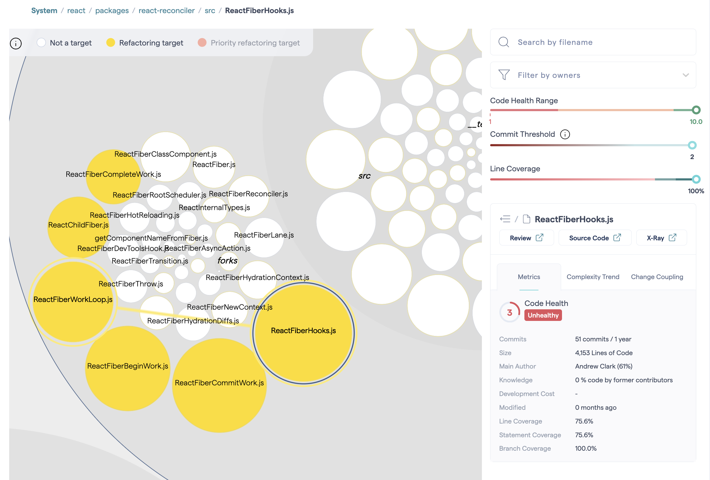
Fig. 182 Refactoring Targets also show code coverage scores to help you evaluate the risk before refactoring.
In addition, the current coverage score for a selected file is visible across other Technical Debt tabs (for example, Hotspots and Refactoring Targets), so you have the same context as you switch perspectives.
Multi-project Code Coverage overview
CodeScene also provides an overview of Code Coverage for all of your projects in the Software Portfolio. It allows you to assess Code Coverage across your entire organization and to make high-level prioritizations.
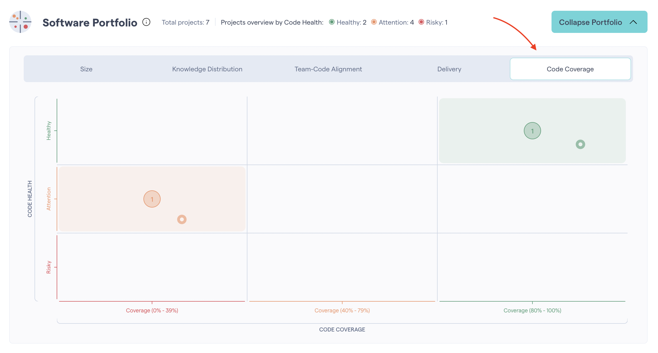
Fig. 183 The Software Portfolio gives an overview of Code Coverage for all projects.
How is average Code Coverage calculated?
Average Code Coverage can be observed on the Software Portfolio and in the interactive Technical Debt map (Code → Technical Debt) under the Summary tab.
The average coverage is calculated as following:
average = covered_lines_from_all_files / total_lines_from_all_files
Metric |
Definition |
|---|---|
|
The total number of lines covered, based on the uploaded coverage data.
The ‘all files’ total refers to the sum of lines across all files
included in the uploaded data. For example, if you upload coverage data
for three files containing 5, 10, and 15 lines respectively, the total
number of lines covered would be 5 + 10 + 15 = 30.
|
|
The total number of executable lines across all files in the codebase.
This includes files for which the coverage data was uploaded, as well
as files that can be parsed by our Xray tool. (Note: files may also be
excluded by the Exclusions and filters project settings)
For example, if the codebase has 6 files: 3 files from the uploaded
coverage data containing 10, 20, and 30 executable lines respectively,
1 file supported by Xray with 50 executable lines, 1 unsupported file
and 1 excluded file, the total would be: 10 + 20 + 30 + 50 = 110.
|